We well be working to classify images as either cats or dogs using a binary perceptron classifier.
1) Perceptron Introduction
The perceptron network consists of the input nodes, that are matched to weights. The network is a dot product of the node vector and the weight vector.
2) Packages
Let’s first import all of the packages we need for this assignment.
-
tensorflow is what we will use to build our neural networks
-
matplotlib helps to plot data and visualize the data
-
numpy helps us make our training and test set arrays
-
keras helps us to make our neural networks
#Author: Leila Abdelrahman
#Adapted from the Classify Images of Clothing Website by François Chollet, 2017, MIT
#Adapted from https://visualstudiomagazine.com/Articles/2013/04/01/Classification-Using-Perceptrons.aspx?Page=1
#Adapted from https://machinelearningmastery.com/implement-perceptron-algorithm-scratch-python/


#Import TensorFlow and Keras
import tensorflow as tf
from tensorflow import keras

#Helper libraries
import numpy as np
import matplotlib.pyplot as plt
from PIL import Image
import cv2
3) Download the Bird and Fish Training Set
Download the BirdvFish data folder and store in the Downloads Folder on the localdisk
4) Designate the destination folder for the photos.
This is done by creating a new direcotory with subdirectories for the train and test set
# organize dataset into a useful structure
from os import makedirs
from os import listdir
from shutil import copyfile
from random import seed
from random import random


# organize dataset into a useful structure
from os import makedirs
from os import listdir
from shutil import copyfile
from random import seed
from random import random
# create directories
dataset_home = 'Downloads/BirdsvFishValidation/'
subdirs = ['train/', 'test/']
for subdir in subdirs:
    # create label subdirectories
    labeldirs = ['birds/', 'fish/']
    for labldir in labeldirs:
        newdir = dataset_home + subdir + labldir
        makedirs(newdir, exist_ok=True)
5) Split the data into training and test sets
Parse through the original source directory and add the respective files into their respective destination directories.
This process is done randomly
The val_ratio determines what ratio of the photos will be used as the test set
# seed random number generator
seed(1)
# define ratio of pictures to use for validation
val_ratio = 0.25
# copy training dataset images into subdirectories
src_directory = 'Downloads/BirdsvFish'
for file in listdir(src_directory):
    src = src_directory + '/' + file

    dst_dir = 'train/'
    if random() < val_ratio:
        dst_dir = 'test/'
    if file.startswith('bird'):
        dst = dataset_home + dst_dir + 'birds/'  + file
        copyfile(src, dst)
    elif file.startswith('fish'):
        dst = dataset_home + dst_dir + 'fish/'  + file
        copyfile(src, dst)
6) Make a class label array to match numbers to class names
class_names = ['bird', 'fish']
7) Rescale the images and read into a directory iterator
Normalization helps to increase speed and accuracy of the model. Divide the images by 255 to generate new rescaled pixels with values between 0 and 1.
Then, convert the directories into arrays.
from keras.preprocessing.image import ImageDataGenerator

batch_size = 39

datagen = ImageDataGenerator(rescale= 1/255)

#training directory iterator
train_it = datagen.flow_from_directory('Downloads/BirdsvFishValidation/train/',
	class_mode='binary', batch_size = batch_size , target_size=(200, 200))


#testing directory iterator
test_it = datagen.flow_from_directory('Downloads/BirdsvFishValidation/test/',
	class_mode='binary', batch_size= batch_size, target_size=(200, 200))

#Convert to arrays
x, y = train_it.next()
X, Y = test_it.next()
Found 105 images belonging to 2 classes.
Found 39 images belonging to 2 classes.
8) Convert to 2D color scale and flatten
-
Convert to 1 color bin Now, parse through the arrays and convert the 3 bins used for colors to 1 bin.
-
Flatten to a 2D array We want to use a linear classifier, so convert the 2D images to a 1 dimentional array/
train_photos = list()
test_photos = list()


#Train data conversion


for i in range (len(y) - 1):
    #convert to grayscale

    photo = cv2.cvtColor(x[i], cv2.COLOR_BGR2GRAY)
    #flatten
    flat = photo.reshape(-1)
    #Add to new list
    train_photos.append(flat)

#Test data conversion

for i in range(len(Y) - 1):

    #convert to grayscale
    photo = cv2.cvtColor(X[i], cv2.COLOR_BGR2GRAY)
    #flatten
    flat = photo.reshape(-1)
    #Add to new list
    test_photos.append(flat)


#Convert lists to arrays

test_photos = np.asarray(test_photos, dtype=np.float32)
train_photos = np.asarray(train_photos, dtype=np.float32)

train_labels = y

test_labels = Y
9) Make the model
- Error minimization using gradient descent
Here we will be using a process using gradient descent to minimize the error. This is done by changing the values of the weights as the function trains and updating them during each epoch.
# Make a prediction with weights

import sys
def Error(train, weights, pixel, bias):

    sum = 0.0;
    for j in range (len(train) - 1):
        sum += train[j] * weights[j]
        sum += bias

    return 0.5 * (sum - pixel) * (sum - pixel)


def TotalError(train,  weights, train_labels, bias):

    totErr = 0.0
    for i in range (len(train) - 1):
        totErr += Error(train[i], weights, train_labels[i], bias)
    return totErr;
10) The Activation Function
The activation function in the perceptron algorithm is a Heave-side step function. If the value of the sum of the weights is negative, the prediction will return 0, meaning the model “thinks” the animal is a bird. If the value of the weights is negative, the function will return 1, meaning that the model “thinks” the animal is a fish.
def predict(row, weights, bias):

    activation = weights[0]
    for i in range(len(row)-1):
        activation += weights[i + 1] * row[i]
        activation += bias
    return 1.0 if activation >= 0.0 else 0.0
11) Working with Weights
- Now we want to change the value of the weights based on the error. We update the weights when we get a mismatch between what the model predicts and what the true class labels are
- The bias is another addition to the model. Think of it as a y intercept in our linear prediction.
# Estimate Perceptron weights using stochastic gradient descent
def train_weights(train, train_labels, l_rate, n_epoch, bias):
    f = 0
    numWeights = len(train[0])
    bestBias = 0.0;
    bias = 0.01;
    smallest_error_so_far = sys.maxsize
    weights = [0.0 for i in range(len(train[0]))]
    best_weights = [0.0 for i in range(len(train[0]))]

    for epoch in range(n_epoch):
        sum_error = 0.0
        for row in train:
            prediction = predict(row, weights, bias)
            desired = train_labels[f]
            delta = desired - prediction
            if prediction != desired:
                for j in range (numWeights - 1):
                    weights[j] = weights[j] +  (l_rate * delta * train[f][j])

                bias = bias + (l_rate * delta)


                totalError = TotalError(train, weights, train_labels, bias)


                if totalError < smallest_error_so_far:
                    smallest_error_so_far = totalError
                    best_weights = weights
                    bestBias = bias
        f += 1


        print('>epoch=%d, lrate=%.3f, error=%.3f' % (epoch, l_rate, smallest_error_so_far))
    return best_weights
12) The Perceptron Algorithm
# Perceptron Algorithm With Stochastic Gradient Descent


def perceptron(train, train_labels, test,test_labels, l_rate, n_epoch, bias):
	predictions = list()
	weights = train_weights(train, train_labels, l_rate, n_epoch, bias)
	for row in test:
		prediction = predict(row, weights, bias)
		predictions.append(prediction)
	return(predictions)
13) Find the Accuracy of the model
bias = 0.01
n_epoch = 20
l_rate = 0.1
def accuracy_metric(actual, predicted):
    correct = 0
    for i in range(len(actual) - 1):
        if actual[i] == predicted[i]:
            correct += 1
    return correct / float(len(actual)) * 100.0


predictions = perceptron(train_photos, train_labels, test_photos, test_labels, l_rate, n_epoch, bias)

print(accuracy_metric(test_labels, predictions))
>epoch=0, lrate=0.100, error=9223372036854775808.000
>epoch=1, lrate=0.100, error=284253641.166
>epoch=2, lrate=0.100, error=5940305.596
>epoch=3, lrate=0.100, error=5940305.596
>epoch=4, lrate=0.100, error=5940305.596
>epoch=5, lrate=0.100, error=5940305.596
>epoch=6, lrate=0.100, error=5940305.596
>epoch=7, lrate=0.100, error=5940305.596
>epoch=8, lrate=0.100, error=5940305.596
>epoch=9, lrate=0.100, error=5940305.596
>epoch=10, lrate=0.100, error=5940305.596
>epoch=11, lrate=0.100, error=5940305.596
>epoch=12, lrate=0.100, error=5940305.596
>epoch=13, lrate=0.100, error=5940305.596
>epoch=14, lrate=0.100, error=5940305.596
>epoch=15, lrate=0.100, error=5940305.596
>epoch=16, lrate=0.100, error=5940305.596
>epoch=17, lrate=0.100, error=5940305.596
>epoch=18, lrate=0.100, error=5940305.596
>epoch=19, lrate=0.100, error=5940305.596
92.3076923076923
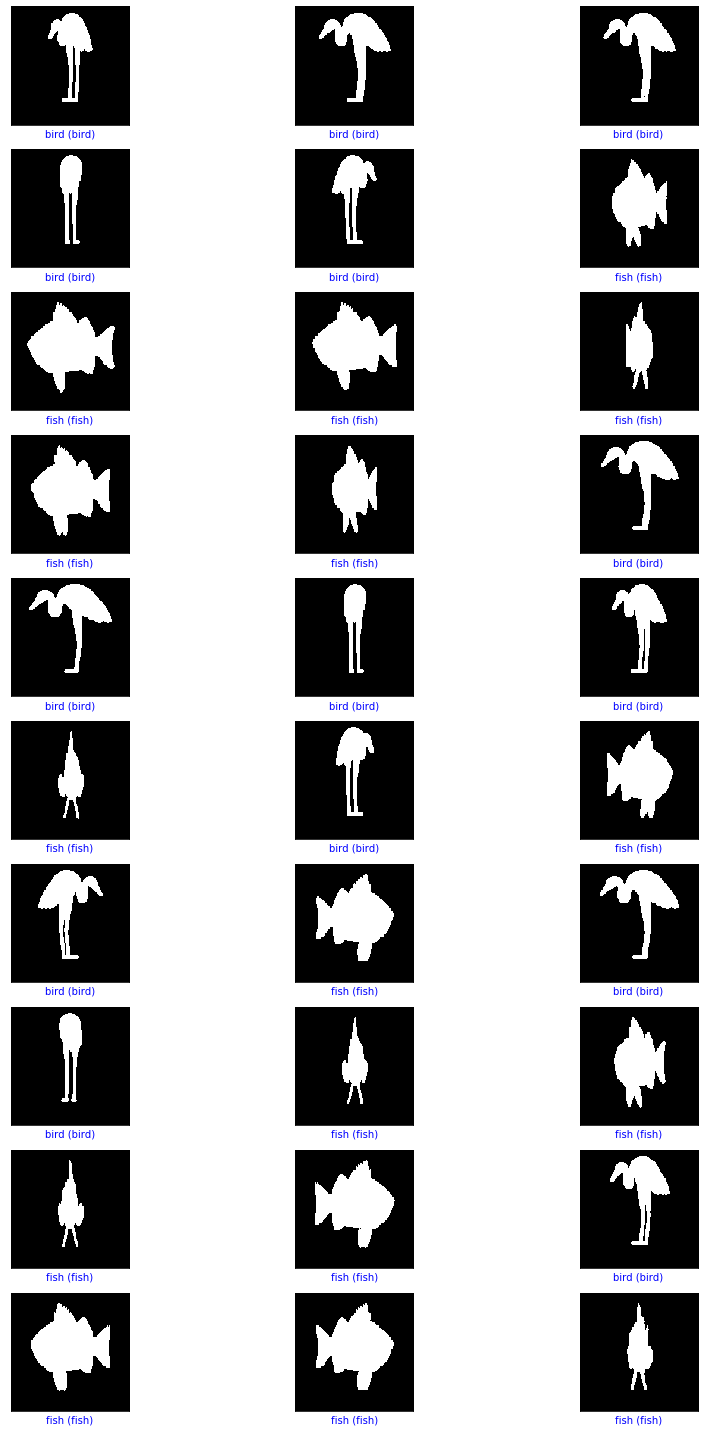
14) Let’s plot the pictures with the predicted and actual class
def plot_image(i , predictions, true_label, img) :
    prediction, true_label, img = predictions[i], int(true_label[i]), img[i]
    plt.grid(False)
    plt.xticks([])
    plt.yticks([])

    plt.imshow(img, cmap=plt.cm.binary)

    predicted_label = int(prediction)
    if predicted_label == true_label:
        color = 'blue'
    else :
        color = 'red'

    plt.xlabel("{} ({})".format(class_names[predicted_label],
                                class_names[int(true_label)]),
                                color=color)
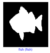
#Now lets look at the 3rd image
i = 2
plt.figure(figsize = (6,3))
plt.subplot(1,2,1)
plot_image(i , predictions, Y, X)

#Now lets look at the 12th image
i = 6
plt.figure(figsize = (6,3))
plt.subplot(1,2,1)
plot_image(i , predictions, Y, X)
#Now let's plot several images with their predictions
#Correct predictions are in blue. Incorrect predictions are in red.

num_rows = 10
num_cols = 3
num_images = num_rows*num_cols
plt.figure(figsize=(2*2*num_cols, 2*num_rows))
for i in range(num_images) :
    plt.subplot(num_rows, 2*num_cols, 2*i+1)
    plot_image(i, predictions, Y, X)
plt.tight_layout()
plt.show()
15) Now It’s Your Turn!
Change your learning rate and see how that affects the model’s accuracy
16) Change the image sources.
You can download a variety of images from ‘https://archive.ics.uci.edu/ml/datasets.php' and modify the direcotory names and classification array names such that you can work with other data sets
# Modify this code:


# create directories
dataset_home = 'Downloads/Lab4SolutionsDataSetValidation/'
subdirs = ['train/', 'test/']
for subdir in subdirs:
    # create label subdirectories
    labeldirs = ['television/', 'teddy/']
    for labldir in labeldirs:
        newdir = dataset_home + subdir + labldir
        makedirs(newdir, exist_ok=True)


# seed random number generator
seed(1)
# define ratio of pictures to use for validation
val_ratio = 0.25
# copy training dataset images into subdirectories
src_directory = r"Desktop/UM Deep Learning Tutorials/Lab4SolutionsData"
for file in listdir(src_directory):
    src = src_directory  + '/' + file

    dst_dir = 'train/'
    if random() < val_ratio:
        dst_dir = 'test/'
    if file.startswith('television'):
        dst = dataset_home + dst_dir + 'television/'  + file
        copyfile(src, dst)
    elif file.startswith('teddy'):
        dst = dataset_home + dst_dir + 'teddy/'  + file
        copyfile(src, dst)


class_names = ['teddy', 'television']
17) Convert to directories and flatten
#Modify the batch size here
batch_size = 39

datagen = ImageDataGenerator(rescale= 1/255)

#training directory iterator
train_it = datagen.flow_from_directory('Downloads/Lab4SolutionsDataSetValidation/train/',
	class_mode='binary', batch_size = batch_size , target_size=(200, 200))


#testing directory iterator
test_it = datagen.flow_from_directory('Downloads/Lab4SolutionsDataSetValidation/test/',
	class_mode='binary', batch_size= batch_size, target_size=(200, 200))

#Convert to arrays
x, y = train_it.next()
X, Y = test_it.next()

train_photos = list()
test_photos = list()


#Train data conversion


for i in range (len(y) - 1):
    #convert to grayscale

    photo = cv2.cvtColor(x[i], cv2.COLOR_BGR2GRAY)
    #flatten
    flat = photo.reshape(-1)
    #Add to new list
    train_photos.append(flat)

#Test data conversion

for i in range(len(Y) - 1):

    #convert to grayscale
    photo = cv2.cvtColor(X[i], cv2.COLOR_BGR2GRAY)
    #flatten
    flat = photo.reshape(-1)
    #Add to new list
    test_photos.append(flat)


#Convert lists to arrays

test_photos = np.asarray(test_photos, dtype=np.float32)
train_photos = np.asarray(train_photos, dtype=np.float32)

train_labels = y

test_labels = Y
Found 105 images belonging to 2 classes.
Found 39 images belonging to 2 classes.
18) Change the bias and learning rate
# PLay around with these and see how they affect training accuracy and the model's computing sped

bias = 0.001
n_epoch = 5
l_rate = 0.01

predictions1 = perceptron(train_photos, train_labels, test_photos, test_labels, l_rate, n_epoch, bias)

print(accuracy_metric(test_labels, predictions1))
>epoch=0, lrate=0.010, error=223982.958
>epoch=1, lrate=0.010, error=223982.958
>epoch=2, lrate=0.010, error=223982.958
>epoch=3, lrate=0.010, error=223982.958
>epoch=4, lrate=0.010, error=223982.958
61.53846153846154
bias = 0.001
n_epoch = 15
l_rate = 0.01

predictions2 = perceptron(train_photos, train_labels, test_photos, test_labels, l_rate, n_epoch, bias)

print(accuracy_metric(test_labels, predictions2))
>epoch=0, lrate=0.010, error=223982.958
>epoch=1, lrate=0.010, error=223982.958
>epoch=2, lrate=0.010, error=223982.958
>epoch=3, lrate=0.010, error=223982.958
>epoch=4, lrate=0.010, error=223982.958
>epoch=5, lrate=0.010, error=223982.958
>epoch=6, lrate=0.010, error=223982.958
>epoch=7, lrate=0.010, error=223982.958
>epoch=8, lrate=0.010, error=223982.958
>epoch=9, lrate=0.010, error=223982.958
>epoch=10, lrate=0.010, error=223982.958
>epoch=11, lrate=0.010, error=223982.958
>epoch=12, lrate=0.010, error=223982.958
>epoch=13, lrate=0.010, error=223982.958
>epoch=14, lrate=0.010, error=223982.958
97.43589743589743
bias = 0.01
n_epoch = 5
l_rate = 0.01

predictions3 = perceptron(train_photos, train_labels, test_photos, test_labels, l_rate, n_epoch, bias)

print(accuracy_metric(test_labels, predictions3))
>epoch=0, lrate=0.010, error=223982.958
>epoch=1, lrate=0.010, error=223982.958
>epoch=2, lrate=0.010, error=223982.958
>epoch=3, lrate=0.010, error=223982.958
>epoch=4, lrate=0.010, error=223982.958
48.717948717948715
bias = 0.01
n_epoch = 20
l_rate = 0.1

predictions4 = perceptron(train_photos, train_labels, test_photos, test_labels, l_rate, n_epoch, bias)

print(accuracy_metric(test_labels, predictions4))
>epoch=0, lrate=0.100, error=401243797.410
>epoch=1, lrate=0.100, error=3331501.776
>epoch=2, lrate=0.100, error=3331501.776
>epoch=3, lrate=0.100, error=3331501.776
>epoch=4, lrate=0.100, error=3331501.776
>epoch=5, lrate=0.100, error=3331501.776
>epoch=6, lrate=0.100, error=3331501.776
>epoch=7, lrate=0.100, error=3331501.776
>epoch=8, lrate=0.100, error=3331501.776
>epoch=9, lrate=0.100, error=3331501.776
>epoch=10, lrate=0.100, error=3331501.776
>epoch=11, lrate=0.100, error=3331501.776
>epoch=12, lrate=0.100, error=3331501.776
>epoch=13, lrate=0.100, error=3331501.776
>epoch=14, lrate=0.100, error=3331501.776
>epoch=15, lrate=0.100, error=3331501.776
>epoch=16, lrate=0.100, error=3331501.776
>epoch=17, lrate=0.100, error=3331501.776
>epoch=18, lrate=0.100, error=3331501.776
>epoch=19, lrate=0.100, error=3331501.776
97.43589743589743
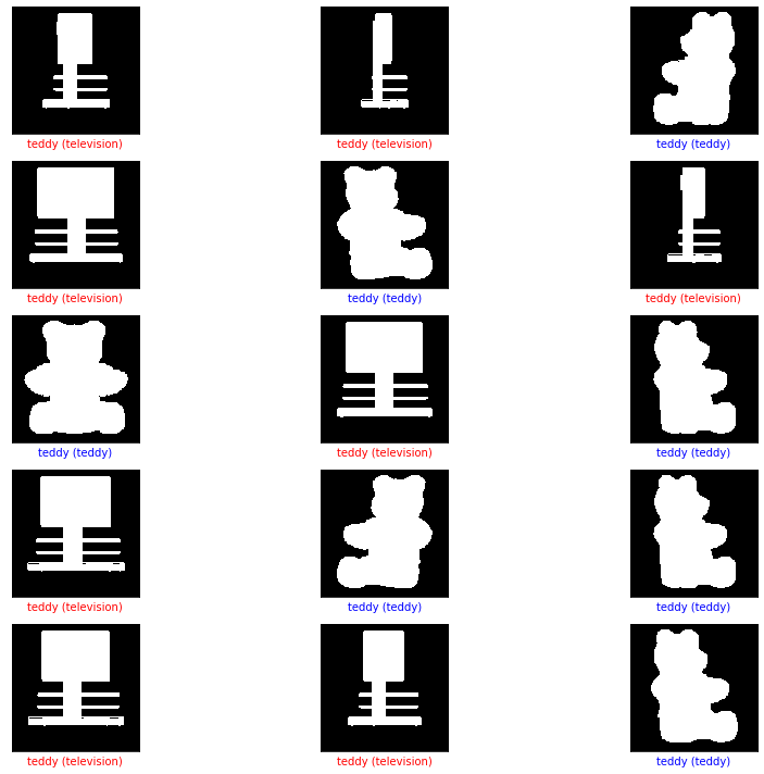
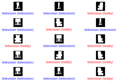
19) Plot images to get a visual representation
# Use the plot function above to plot the images and their predicted class, along with the accurate class.

num_rows = 5
num_cols = 3
num_images = num_rows*num_cols
plt.figure(figsize=(2*2*num_cols, 2*num_rows))
for i in range(num_images) :
    plt.subplot(num_rows, 2*num_cols, 2*i+1)
    plot_image(i, predictions1, Y, X)
plt.tight_layout()
plt.show()
for i in range(num_images) :
    plt.subplot(num_rows, 2*num_cols, 2*i+1)
    plot_image(i, predictions2, Y, X)
plt.tight_layout()
plt.show()
for i in range(num_images) :
    plt.subplot(num_rows, 2*num_cols, 2*i+1)
    plot_image(i, predictions3, Y, X)
plt.tight_layout()
plt.show()
for i in range(num_images) :
    plt.subplot(num_rows, 2*num_cols, 2*i+1)
    plot_image(i, predictions4, Y, X)
plt.tight_layout()
plt.show()
