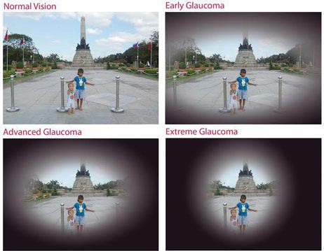
Glaucoma is a disease caused by high intraoccular pressure that leads to degenertation of the optic nerve and visual perspective
Below is an example of the degenerative visual effects of glaucoma
1) Import the necessary libraries
We will be predicitng a advanced, early, and control glaucoma based on eye fundus images.
To begin, we need to right libraries
-
os is what we will use to modify file names and create new directories
-
tensorflow is what we will use to build our neural networks
-
matplotlib helps to plot data and visualize the data
-
numpy helps us make our training and test set arrays
-
keras helps us to make our neural networks
import os

#Import TensorFlow and Keras
import tensorflow as tf
from tensorflow import keras

#Helper libraries
import numpy as np
import matplotlib.pyplot as plt
2) Download the data and create necessary directories
Download the data from here
- Make sure to import additional necessary libraries like random.
# organize dataset into a useful structure
from os import makedirs
from os import listdir
from shutil import copyfile
from random import seed
from random import random


# create directories
dataset_home = 'Downloads/Eye_Fundus_Images_Validation/'
subdirs = ['train/', 'test/']
for subdir in subdirs:
    # create label subdirectories
    labeldirs = ['advanced_glaucoma/', 'early_glaucoma/', 'normal_control/']
    for labldir in labeldirs:
        newdir = dataset_home + subdir + labldir
        makedirs(newdir, exist_ok=True)
3) Split the data into test and training sets
- Define the validation ratio. In this case, we are trainig on 75% of the data and testing on 25%
# seed random number generator
seed(1)
# define ratio of pictures to use for validation
val_ratio = 0.25
# copy training dataset images into subdirectories
src_directory = 'Downloads/Eye_Fundus_Images'

for label in labeldirs:

    new_src_directory = src_directory + '/' + label
    print(new_src_directory)

    for file in listdir(new_src_directory):
        oldFileName = new_src_directory + file

        newFileName = new_src_directory + '/' + label[:-1] + file


        os.rename(oldFileName, newFileName)

        newFileIndividualName = label[:-1] + file

        dst_dir = 'train/'
        if random() < val_ratio:
            dst_dir = 'test/'
        if newFileIndividualName.startswith(label[:-1]):
            dst = dataset_home + dst_dir + label  + newFileIndividualName
            copyfile(newFileName, dst)
Downloads/Eye_Fundus_Images/advanced_glaucoma/
Downloads/Eye_Fundus_Images/early_glaucoma/
Downloads/Eye_Fundus_Images/normal_control/
4) Create a class names array
class_names = ['advanced glaucoma', 'early glaucoma' , 'normal control']
5) Use an image generator to
- rescale the images to a pixel value between 0 and 1.
- generate new, augmented images by horizontally flipping the images
- resize the images to 240*240 pixels
- Also store the information in the iterators as arrays for further processing
from keras.preprocessing.image import ImageDataGenerator


datagen = ImageDataGenerator(
      rescale = 1./255,
      horizontal_flip=True)

#training directory iterator
train_it = datagen.flow_from_directory( dataset_home + 'train/',
	class_mode='categorical', target_size=(240, 240))


#testing directory iterator
test_it = datagen.flow_from_directory(dataset_home + 'test/',
	class_mode='categorical', target_size=(240, 240))

#Convert to arrays
x, y = train_it.next()
X, Y = test_it.next()
Found 1185 images belonging to 3 classes.
Found 359 images belonging to 3 classes.
6) Make the model
This model consists of
- 4 Convolutional layers, each followed by maxpooling
- Every layer regularizes the weights using Xavier regularization
- There are 3 fully connected layers.
- Before connecting to the fully connected layers, we use a dropout function with 0.5
model = keras.Sequential([

    keras.layers.Conv2D(64, (3,3), activation='relu', input_shape=(240, 240, 3), kernel_initializer = 'glorot_normal'),
    keras.layers.MaxPooling2D(2,2),
    # The second convolution
    keras.layers.Conv2D(64, (3,3), activation='relu' , kernel_initializer = 'glorot_normal'),
    keras.layers.MaxPooling2D(2,2),
    keras.layers.Conv2D(128, (3,3), activation='relu' , kernel_initializer = 'glorot_normal'),
    keras.layers.MaxPooling2D(2,2),
    keras.layers.Conv2D(128, (3,3), activation='relu' , kernel_initializer = 'glorot_normal'),
    keras.layers.MaxPooling2D(2,2),
    # Flatten the results to feed into a DNN
    keras.layers.Flatten(),
    keras.layers.Dropout(0.5),
    # 512 neuron hidden layer
    #keras.layers.Dense(512, kernel_initializer = "glorot_uniform") ,
    keras.layers.Dense(32, activation='relu' , kernel_initializer = 'glorot_normal') ,
    keras.layers.Dense(64, activation = 'relu' , kernel_initializer = 'glorot_normal'
                      ) ,
    keras.layers.Dense(3, activation='softmax')
])


model.summary()

model.compile(loss = 'categorical_crossentropy', optimizer='adagrad', metrics=['accuracy'])

history = model.fit_generator(train_it, epochs=25, validation_data = test_it, verbose = 1)
Model: "sequential_3"
_________________________________________________________________
Layer (type)                 Output Shape              Param #
=================================================================
conv2d_12 (Conv2D)           (None, 238, 238, 64)      1792
_________________________________________________________________
max_pooling2d_12 (MaxPooling (None, 119, 119, 64)      0
_________________________________________________________________
conv2d_13 (Conv2D)           (None, 117, 117, 64)      36928
_________________________________________________________________
max_pooling2d_13 (MaxPooling (None, 58, 58, 64)        0
_________________________________________________________________
conv2d_14 (Conv2D)           (None, 56, 56, 128)       73856
_________________________________________________________________
max_pooling2d_14 (MaxPooling (None, 28, 28, 128)       0
_________________________________________________________________
conv2d_15 (Conv2D)           (None, 26, 26, 128)       147584
_________________________________________________________________
max_pooling2d_15 (MaxPooling (None, 13, 13, 128)       0
_________________________________________________________________
flatten_3 (Flatten)          (None, 21632)             0
_________________________________________________________________
dropout_3 (Dropout)          (None, 21632)             0
_________________________________________________________________
dense_7 (Dense)              (None, 32)                692256
_________________________________________________________________
dense_8 (Dense)              (None, 64)                2112
_________________________________________________________________
dense_9 (Dense)              (None, 3)                 195
=================================================================
Total params: 954,723
Trainable params: 954,723
Non-trainable params: 0
_________________________________________________________________
Epoch 1/25
WARNING:tensorflow:From C:\Users\coder\Anaconda3\envs\TensorFlow\lib\site-packages\tensorflow_core\python\keras\optimizer_v2\adagrad.py:107: calling Constant.__init__ (from tensorflow.python.ops.init_ops) with dtype is deprecated and will be removed in a future version.
Instructions for updating:
Call initializer instance with the dtype argument instead of passing it to the constructor


37/38 [============================>.] - ETA: 2s - loss: 0.9074 - acc: 0.5950Epoch 1/25
38/38 [==============================] - 114s 3s/step - loss: 0.8999 - acc: 0.6008 - val_loss: 0.7370 - val_acc: 0.6992
Epoch 2/25
37/38 [============================>.] - ETA: 2s - loss: 0.6713 - acc: 0.7025Epoch 1/25
38/38 [==============================] - 113s 3s/step - loss: 0.6763 - acc: 0.6987 - val_loss: 0.6985 - val_acc: 0.7047
Epoch 3/25
37/38 [============================>.] - ETA: 2s - loss: 0.7061 - acc: 0.6895Epoch 1/25
38/38 [==============================] - 114s 3s/step - loss: 0.7096 - acc: 0.6861 - val_loss: 0.7560 - val_acc: 0.6657
Epoch 4/25
37/38 [============================>.] - ETA: 2s - loss: 0.6705 - acc: 0.7042Epoch 1/25
38/38 [==============================] - 113s 3s/step - loss: 0.6669 - acc: 0.7055 - val_loss: 0.6312 - val_acc: 0.7298
Epoch 5/25
37/38 [============================>.] - ETA: 2s - loss: 0.6216 - acc: 0.7112Epoch 1/25
38/38 [==============================] - 112s 3s/step - loss: 0.6181 - acc: 0.7139 - val_loss: 0.6163 - val_acc: 0.7354
Epoch 6/25
37/38 [============================>.] - ETA: 2s - loss: 0.6287 - acc: 0.7190Epoch 1/25
38/38 [==============================] - 112s 3s/step - loss: 0.6338 - acc: 0.7156 - val_loss: 0.8917 - val_acc: 0.5543
Epoch 7/25
37/38 [============================>.] - ETA: 2s - loss: 0.6188 - acc: 0.7259Epoch 1/25
38/38 [==============================] - 113s 3s/step - loss: 0.6167 - acc: 0.7274 - val_loss: 0.6232 - val_acc: 0.7437
Epoch 8/25
37/38 [============================>.] - ETA: 2s - loss: 0.5830 - acc: 0.7251Epoch 1/25
38/38 [==============================] - 114s 3s/step - loss: 0.5848 - acc: 0.7266 - val_loss: 0.6059 - val_acc: 0.7382
Epoch 9/25
37/38 [============================>.] - ETA: 2s - loss: 0.6555 - acc: 0.7173Epoch 1/25
38/38 [==============================] - 114s 3s/step - loss: 0.6553 - acc: 0.7148 - val_loss: 0.6076 - val_acc: 0.7493
Epoch 10/25
37/38 [============================>.] - ETA: 2s - loss: 0.5799 - acc: 0.7355Epoch 1/25
38/38 [==============================] - 114s 3s/step - loss: 0.5825 - acc: 0.7342 - val_loss: 0.6506 - val_acc: 0.7187
Epoch 11/25
37/38 [============================>.] - ETA: 2s - loss: 0.6558 - acc: 0.7138Epoch 1/25
38/38 [==============================] - 112s 3s/step - loss: 0.6545 - acc: 0.7131 - val_loss: 0.6354 - val_acc: 0.7521
Epoch 12/25
37/38 [============================>.] - ETA: 2s - loss: 0.6003 - acc: 0.7348Epoch 1/25
38/38 [==============================] - 111s 3s/step - loss: 0.6295 - acc: 0.7342 - val_loss: 0.6961 - val_acc: 0.6602
Epoch 13/25
37/38 [============================>.] - ETA: 2s - loss: 0.5906 - acc: 0.7398Epoch 1/25
38/38 [==============================] - 111s 3s/step - loss: 0.5895 - acc: 0.7384 - val_loss: 0.6284 - val_acc: 0.7493
Epoch 14/25
37/38 [============================>.] - ETA: 2s - loss: 0.5707 - acc: 0.7389Epoch 1/25
38/38 [==============================] - 112s 3s/step - loss: 0.5738 - acc: 0.7350 - val_loss: 0.6031 - val_acc: 0.7437
Epoch 15/25
37/38 [============================>.] - ETA: 2s - loss: 0.5726 - acc: 0.7320Epoch 1/25
38/38 [==============================] - 111s 3s/step - loss: 0.5747 - acc: 0.7300 - val_loss: 0.6104 - val_acc: 0.7131
Epoch 16/25
37/38 [============================>.] - ETA: 2s - loss: 0.5765 - acc: 0.7389Epoch 1/25
38/38 [==============================] - 112s 3s/step - loss: 0.5740 - acc: 0.7401 - val_loss: 0.5782 - val_acc: 0.7437
Epoch 17/25
37/38 [============================>.] - ETA: 2s - loss: 0.6235 - acc: 0.7407Epoch 1/25
38/38 [==============================] - 116s 3s/step - loss: 0.6212 - acc: 0.7409 - val_loss: 0.5976 - val_acc: 0.7382
Epoch 18/25
37/38 [============================>.] - ETA: 2s - loss: 0.6068 - acc: 0.7528Epoch 1/25
38/38 [==============================] - 114s 3s/step - loss: 0.6034 - acc: 0.7544 - val_loss: 0.5938 - val_acc: 0.7577
Epoch 19/25
37/38 [============================>.] - ETA: 2s - loss: 0.5923 - acc: 0.7459Epoch 1/25
38/38 [==============================] - 113s 3s/step - loss: 0.5916 - acc: 0.7460 - val_loss: 0.5792 - val_acc: 0.7493
Epoch 20/25
37/38 [============================>.] - ETA: 2s - loss: 0.5736 - acc: 0.7346Epoch 1/25
38/38 [==============================] - 113s 3s/step - loss: 0.5723 - acc: 0.7376 - val_loss: 0.5896 - val_acc: 0.7549
Epoch 21/25
37/38 [============================>.] - ETA: 2s - loss: 0.5867 - acc: 0.7407Epoch 1/25
38/38 [==============================] - 113s 3s/step - loss: 0.5851 - acc: 0.7426 - val_loss: 0.5850 - val_acc: 0.7242
Epoch 22/25
37/38 [============================>.] - ETA: 2s - loss: 0.5800 - acc: 0.7502Epoch 1/25
38/38 [==============================] - 115s 3s/step - loss: 0.5785 - acc: 0.7511 - val_loss: 0.5861 - val_acc: 0.7354
Epoch 23/25
37/38 [============================>.] - ETA: 2s - loss: 0.5584 - acc: 0.7520Epoch 1/25
38/38 [==============================] - 114s 3s/step - loss: 0.5609 - acc: 0.7519 - val_loss: 0.5837 - val_acc: 0.7577
Epoch 24/25
37/38 [============================>.] - ETA: 2s - loss: 0.5614 - acc: 0.7450Epoch 1/25
38/38 [==============================] - 115s 3s/step - loss: 0.5627 - acc: 0.7460 - val_loss: 0.5843 - val_acc: 0.7632
Epoch 25/25
37/38 [============================>.] - ETA: 2s - loss: 0.5483 - acc: 0.7546Epoch 1/25
38/38 [==============================] - 115s 3s/step - loss: 0.5475 - acc: 0.7544 - val_loss: 0.5899 - val_acc: 0.7354
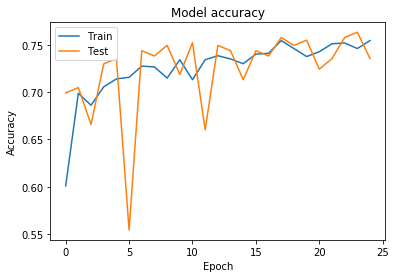
7) Plot the training and validation accuracy
# Plot training & validation accuracy values
plt.plot(history.history['acc'])
plt.plot(history.history['val_acc'])
plt.title('Model accuracy')
plt.ylabel('Accuracy')
plt.xlabel('Epoch')
plt.legend(['Train', 'Test'], loc='upper left')
plt.show()
8) Test the model on the testing data
predicitions = model.predict_generator(test_it)
loss, acc = model.evaluate_generator(test_it)
9) Print the model’s accuracy on the test data
print("The model's accuracy on the test data is: " + str(acc))
The model's accuracy on the test data is: 0.73816156
10) Define functions for plotting the image and the probability value array
import matplotlib.pyplot as plt

def plot_image(i , predictions_array, true_label, img) :
    predictions_array, true_label, img = predictions_array, true_label[i], img[i]
    plt.grid(False)
    plt.xticks([])
    plt.yticks([])

    plt.imshow(img, cmap=plt.cm.binary)

    predicted_label = np.argmax(predictions_array)

    true_label_index = np.argmax(true_label)
    predited_label = np.argmax(predictions_array)
    if predicted_label == true_label_index:
        color = 'blue'
    else :
        color = 'red'

    plt.xlabel("{} {:2.0f}% ({})".format(class_names[predicted_label],
                                100*np.max(predictions_array),
                                class_names[true_label_index]),
                                color=color)

def plot_value_array(i, predictions_array, true_label) :
    predictions_array, true_label = predictions_array, true_label[i]
    plt.grid(False)
    plt.xticks(range(3))
    plt.yticks([])
    thisplot = plt.bar(range(3), predictions_array , color = "#777777")
    plt.ylim([0,1])
    predicted_label = np.argmax(predictions_array)

    true_label_index = np.argmax(true_label)

    thisplot[predicted_label].set_color('red')
    thisplot[true_label_index].set_color('blue')
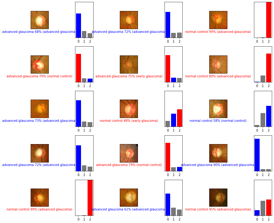
11) Now let’s plot several images with their predictions
Correct predictions are in blue. Incorrect predictions are in red.
num_rows = 5
num_cols = 3
num_images = num_rows*num_cols
plt.figure(figsize=(2*2*num_cols, 2*num_rows))
for i in range(num_images) :
    plt.subplot(num_rows, 2*num_cols, 2*i+1)
    plot_image(i, predicitions[i], Y, X)
    plt.subplot(num_rows, 2*num_cols, 2*i+2)
    plot_value_array(i, predicitions[i], Y)
plt.tight_layout()
plt.show()
Resources
- https://dataverse.harvard.edu/dataset.xhtml?persistentId=doi:10.7910/DVN/1YRRAC
- https://keras.io/visualization/
- Adapted from the Classify Images of Clothing Website by François Chollet, 2017, MIT
- https://journals.plos.org/plosone/article?id=10.1371%2Fjournal.pone.0207982